Tilt-series to tomograms
Contents
Tilt-series to tomograms#
In this section we will
align our tilt-series
perform a more accurate tilt-series CTF estimation procedure
reconstruct our tomograms at 10 Å/px
Tilt-series alignment#
To align our tilt-series we will use the autoalign_dynamo package, which leverages Dynamo’s automated tilt series alignment workflows.
This program aligns tilt-series in Dynamo and prepares all necessary metadata for import back into Warp.
Overview#
Basic overview of the tilt-series alignment procedure in Dynamo:
Estimation of the putative positions of fiducials in all the images by cross-correlation (CC) against a synthetic template.
Rejection of features that are not rotationally symmetric, and therefore likely not beads.
Indexing of bead observations, attempting to determine which beads correspond to the same underlying object in 3D.
Iterative refinement of the alignment parameters and bead positions.
Reintegration of missing observations based on an updated projection model.
Removal of observations with large residuals.
This procedure explicitly attempts to maximise the number of observations which should increase the global accuracy of the final solution.
To enable use of these workflows within the Warp preprocessing pipeline we provide a package autoalign_dynamo. dautoalign4warp is a function provided by this package which handles running the Dynamo alignment workflow on all tilt-series and prepares all metadata for import back into Warp. This procedure can be run on-the-fly, starting as soon as the first tilt-series has been generated by Warp.
Aligning the tilt-series#
Open MATLAB, make sure that dynamo and autoalign_dynamo are activated and navigate to the frames directory.
The command we need to use is:
dautoalign4warp(<warp_tilt_series_directory>, <pixel_size_angstrom>, <fiducial_diameter_nm>, <nominal_rotation_angle>, <output_folder>)
Warp puts the generated tilt series in a new imod directory, one level below the frames directory.
For this dataset the fiducial diameter is 10 nm and the nominal rotation angle is 85.3 degrees.
We can start aligning tilt-series with the following command:
dautoalign4warp('./imod', 1.35, 10, 85.3, './dynamo_alignments')
This command will generate the transforms needed to align a tilt series
Once running, autoalign_dynamo will keep processing incoming data from Warp and generate the metadata necessary for tomogram reconstruction.
As soon as the alignments are done, we can start CTF estimation on the tilt-series and reconstructing tomograms.
Checking the results#
In the dynamo_alignments folder there is a .mod file in a folder for each tilt-series.
This model file can be opened with the tilt-series in 3dmod to visually check that the beads have been detected and tracked appropriately.
The taSolution.log file also contains useful information about the quality of the alignments.
Tilt-Series CTF Estimation and Tomogram reconstruction#
Up to now we have:
preprocessed the 2D images
generated and aligned tilt-series
We will now estimate the CTF parameters for each tilt-series, check that our CTF model has the correct handedness and reconstruct the tomograms.
Import aligned tilt-series#
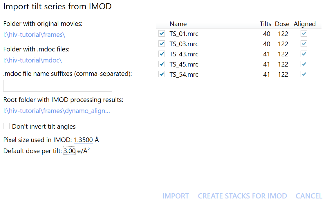
To import the newly aligned tilt series back into Warp, click the import tilt series from IMOD button and select the frames and mdoc folders as before. Then, set Root folder with IMOD processing results to the new dynamo_alignments directory.
The checkboxes should now appear checked in the Aligned column on the right hand side of the import window.
Differently from earlier, now we also need to enter the pixel size of the tilt-series and the electron dose that the sample was exposed to per tilt.
For this dataset this is the binned pixel size of 1.35 \(Å/px\), and according the the EMPIAR entry the dose is roughly 3 \(e^-/Å^2\) per tilt.
Tilt-Series CTF estimation#
In this step, Warp will reestimate the CTF parameters for each tilt series according to a 3D model of the underlying signal which accounts for defocus variations due to tilt angle, sample thickness and sample inclination relative to the imaging plane. Using this 3D model, individual particles can be reconstructed from images which have been CTF corrected according to their exact position within the reconstructed volume.
Check tilt handedness#
The tilt handedness check allows us to check that defocus varies across each image as expected by Warp’s CTF model for each tilt-series.
To perform the check, we first estimate the CTF for one tilt-series by hitting estimate for just this tilt-series in the Fourier Space tab. Once this has completed, we have to hit Check tilt handedness. If Warp sees that the defocus estimates don’t match what it expects in terms of how the defocus changes with tilt-angle, it will offer the option to flip the defocus handedness of the CTF model for each loaded tilt-series. If the correlation found is not convincing, try other tilt-series in the dataset.
Once we are sure about the tilt handedness, we can proceed with the tilt-series CTF estimation procedure.
CTF estimation#
The settings for tilt-series CTF estimation should be the same as those used earlier when estimating CTF parameters for 2D micrographs. In this case, we do not control the spatiotemporal resolution of the CTF model. Simply click on START PROCESSING to proceed.
Reconstruct tomograms#
We now have everything we need to reconstruct our tomograms. In Warp, we don’t need to reconstruct whole tomograms at this step. Instead, downsampled tomograms can be generated for initial particle picking and volumes centered on each object of interest can be reconstructed later at the desired pixel size. This reduces the computational burden of generating and extracting particles from large, unbinned tomograms which can easily be over 100GB in size.
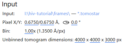
We have to define the reconstruction area by setting the Unbinned tomogram dimensions. These are the dimensions that the tomogram would have if reconstructed at the pixel size of the unbinned tilt images. To capture the full extent of the imaged area, we should use 8000 x 8000 for the x and y dimensions. In z, we want the reconstruction to be large enough to include the entire imaged sample. In this case, 6000 \(px\) is more than enough.
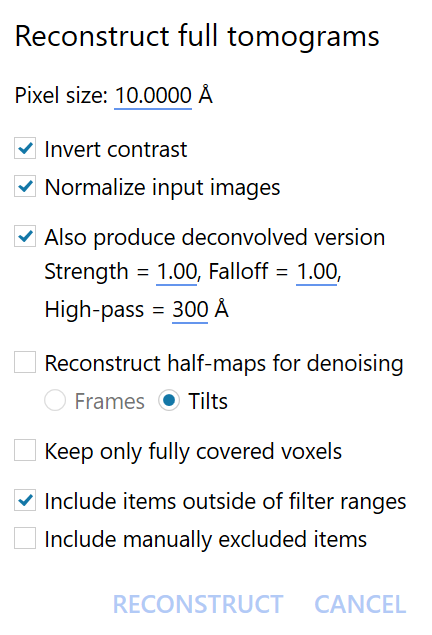
We can then click on reconstruct full tomograms at the top of the Overview tab to open the reconstruction dialog box.
We invert contrast such that any averages of particles in the tomograms will be light-on-dark. Whilst not strictly necessary, this is a convention which facilitates visualisation in programs such as ChimeraX and the use of certain image processing tools which expect this inverted contrast.
We also select Also produce deconvolved version; this generates a tomogram which has been filtered for visualisation alongside the unfiltered reconstruction suitable for subtomogram averaging.
Leave Reconstruct half-maps for denoising and Keep only fully covered voxels unchecked for now, the first is useful if you want to denoise your data and the second will leave zeros in the regions not contributed to by all images in the tilt-series.
Warp may have marked some tilt series as filtered out. Since we are not making active use of filters in this tutorial, this is not a problem. Simply select Include items outside of filter ranges. To learn more about the Warp filters, check out the Warp tutorial on frame series.
Once ready, click on Reconstruct to reconstruct the tomograms.