Particle pose optimisation
Contents
Particle pose optimisation#
Now that we have a set of particles that’s mostly free of duplicates and matches our geometrical understanding of the system, we can proceed to refine of our particle poses with the aim of producing a higher resolution average.
In this section, we will:
Extract particles in Warp at 5Å/px
Align these particles by subtomogram averaging in RELION
Repeat the previous two steps at 1.6Å/px
Tip
Subtomogram averaging becomes very slow when performing refinements with lots of particles in larger boxes. Stepping the pixel size down gradually allows us to move more quickly and react to any problems which may come up when working on more complex data.
Reconstruct subtomograms in Warp at 5Å/px#
Generate compatible metadata#
Our metadata is currently in the dynamo format.
We need to convert our particle positions and orientations into a format Warp understands, we will use the dynamo2warp script provided by the
dynamo2m
package. The script takes a .tbl file (which we generated at the end of the previous section) and a table map file. The table map file contains a mapping from particle indexes to file names, to match to the column 20 of the .tbl file. In our case, this file is located in dynamo/findparticlesData.Boxes/indices_column20.doc.
In a terminal, run:
dynamo2warp -i result_10Apx_nodup_neighbourcleaning.tbl -tm ../../../../findparticlesData.Boxes/indices_column20.doc -o result_10Apx_nodup_neighbourcleaning_data.star
Subtomogram reconstruction in Warp#
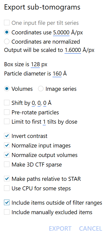
We can now use the generated .star file to reconstruct subtomograms from our tilt-series in Warp. To start the reconstruction, make sure Warp is in *.tomostar mode, then click on the Reconstruct sub-tomograms button at the top of the screen in the Overview tab and select result_10Apx_nodup_neighbourcleaning_data.star. A dialog will open; fill in the settings as follows, making sure the radio buttons all selected correctly:
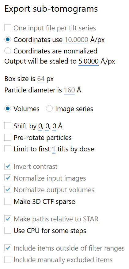
When ready, click on EXPORT. To prepare the directory structure for relion, we will choose to put the output .star file inside a new relion folder in the project root directory, and call it subtomograms_5Apx.star.
3D auto-refine in RELION#
We can now perform a gold standard automatic refinement of the whole dataset at 5Å/px in RELION. Working in RELION at this stage simplifies the workflow and allows us to take advantage of its maximum-likelihood approaches to refinement and classification.
At this stage, we choose not to use a density-based mask during refinement. This allows us to make use of the neighbouring density in the lattice to drive these initial alignments. We will use a mask later when aiming for more precise, local alignment of the central hexamer.
Note
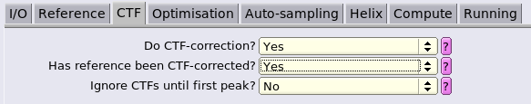
By default, Dynamo uses a binary wedge model to account for the sampling of information in Fourier space for each subtomogram. Warps CTF volumes are designed for use with RELION and should yield more accurate weighting of Fourier coefficients during reconstruction.
Before alignment, we need to create an initial reference for the alignment procedure. We select a random subset of particles with simple bash commands:
# keep the header
head subtomograms_5Apx.star -n 30 > random_subset_5Apx.star
# use 500 random particles
tail subtomograms_5Apx.star -n +31 | shuf -n 500 >> random_subset_5Apx.star
Then, we use relion_reconstruct from the command line to align and average them. We need to make sure to appropriately weight the reconstruction according to the CTF volumes and tell the program that we are working with 3D images.
relion_reconstruct --i random_subset_5Apx.star --o random_subset_5Apx.mrc --3d_rot --ctf --sym C6
This step also serves as a useful sanity check. The resulting reconstruction should look like the hexagonal lattice we have seen previously. If it doesn’t, something went wrong: check your parameters carefully for each step.
Alignment in RELION#
To start the project, run relion from the relion directory.
relion
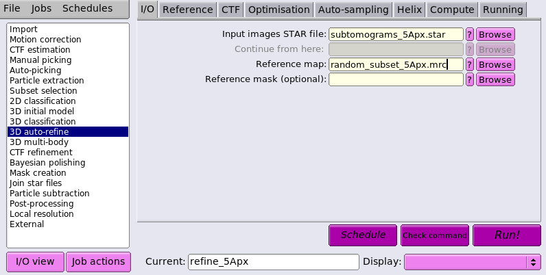
We then set up a 3D auto-refine job as following:
We will refine without a mask for now as this refinement serves only to make sure that the particles remain well centered and we expect to go significantly beyond 10Å.
We use a conservative initial lowpass of 30Å to avoid overfitting, and C6 symmetry based on our understanding of the lattice from the inital model generation.
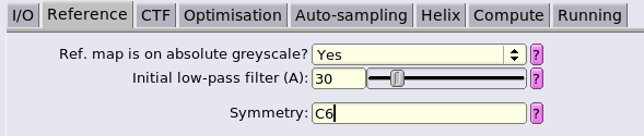
We use a particle diameter covering the whole box to continue making use of the signal from neighbouring hexamers to drive alignment. We will change this once we start aiming for more optimal refinements focussed on the central hexamer.
Leave this disabled, we are not performing helical refinement in this case.
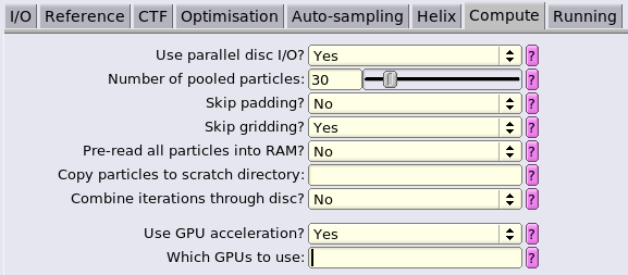
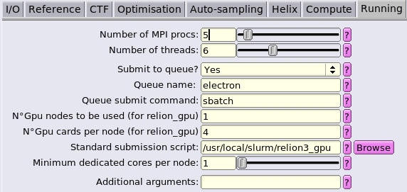
The specific computational parameters will depend upon the configuration of your computing resources. Here, we are running on a cluster node with:
4 x GeForce GTX 1080 TI GPUs
16 x E5-2620 v4 2.10GHz CPUs (2 threads per core)
256GB RAM
and which uses slurm to manage its jobs.
Once ready, click on Run! to start processing. This will take several hours!
Subtomogram reconstruction at 1.6Å/px#
Warning
We reconstructed at 1.6Å/px rather than 1.35Å/px due to memory limitations. Warp works with larger images internally to reduce the effects of CTF aliasing. The large number of particles per field-of-view is particularly demanding at such a small pixel size and can lead to memory issues. Unless working at a very small pixel size, you are unlikely to encounter these issues when working with your own data.
Once the alignment at 5Å/px is done, we can perform alignments at a smaller pixel size to obtain a higher resolution reconstruction. We use Warp to reconstruct sutomograms at 1.6Å/px using the *_data.star from the refinement at 5Å/px then rerun the alignments in Relion. This time, we will perform our refinements in a mask around the central hexamer.
First, we need to reformat the output .star file from the Relion3.1 specification (not supported by Warp 1.0.9) to Relion3.0, using a command provided by dynamo2m. To do so, navigate to relion/Refine3D/refine_5apx and identify the last iteration number (for us, it was it_023) and run:
relion_star_downgrade -s run_it023_data.star
From the new file run_it023_data_rln3.0.star, we can now reconstruct subtomograms in Warp. This time, the input coordinates use 5Å/px and the output should be scaled to 1.6Å/px. To optimise computational speed, we choose a box size of 128 px here. This is a little smaller than our previous box size, but still big enough for our particle.
Attention
Using small box sizes, especially for particles with a large defocus containing fast CTF oscillations, can lead to CTF aliasing. We can use a fairly small box here because Warp implements an aliasing-free reconstruction algorithm to avoid this.
Save the file in the relion directory as subtomograms_1.6Apx.star
Generate a reconstruction at 1.6Å/px using relion_reconstruct with the following command.
relion_reconstruct --i subtomograms_1.6Apx.star --o reconstruction_1.6Apx.mrc --3d_rot --ctf --sym C6
Creating a mask for refinement#
To focus our refinements on the central hexamer, we need to produce a mask around this region. The mask should have a soft edge, this avoids introducing bias into masked FSC calculations, see here for discussion.
To produce our mask we will
produce a map containing only the central hexamer
use this map to generate a soft-edged mask around the central hexamer
We can quickly mask out the central hexamer interactively using tools in Dynamo.
In MATLAB with Dynamo activated, load your reconstruction at 1.6Å/px into an old version of the dynamo_mapview GUI.
dpkdev.legacy.dynamo_mapview('reconstruction_1.6Apx.mrc')
The mask should be a cylinder with a diameter of 160Å around the central hexamer of the lattice. See our mini-tutorial on mask creation for details on creating the mask.
Once you’re happy with the mask, mask your volume and save it as central_hexamer_1.6Apx.mrc from the GUI.
Open your central_hexamer_1.6Apx.mrc in your favourite program and determine an appropriate threshold for binarisation. Use this as the --ini_threshold parameter in the following command.
relion_mask_create --i central_hexamer_1.6Apx.mrc --angpix 1.6 --extend_inimask 5 --width_soft_edge 10 --o mask_1.6Apx.mrc --ini_threshold 0.05
Refinement at 1.6Å/px#
Now that we have a mask, we can set up a relion 3D auto-refine job like we did before. A few parameters require changes:
change the name of the project in
Currentunder theI/Otab to reflect the smaller pixel size; we usedrefine_1.6Apxinputs should now be the
_1.6Apxstar file, reference and mask we generated, respectively:subtomograms_1.6Apx.starreconstruction_1.6Apx.mrcmask_1.6Apx.mrc
the inital low pass filter under the
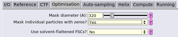
Referencetab can be set up to the estimated resolution from the previous refinement at 5Å/px. This will speed up the convergence of the refinement. In our case, 15 is appropriate.the mask diameter in the
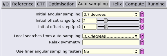
Optimisationtab should be lowered to 160Å to encompass only the central hexamer.the inital and local searched for angular sampling in the
Auto-samplingtab can be restricted to 1.8 degrees.
Leaving the rest as before, press Run! to start processing. Once the processing is done, we are ready to move on to the multi-particle refinement in M.