Geometrical particle picking
Contents
Geometrical particle picking#
The tomograms are reconstructed and ready for further analysis. Warp includes a template matching procedure, but what if we don’t know what our object of interest looks like yet?
In biological systems, particles often have a spatial relationship with an underlying supporting geometry such as a membrane, filament or vescicle.
Exploiting this prior knowledge about the geometry of a system is often useful in subtomogram averaging, reducing both the computational burden and the risk of particles ending up in obviously wrong positions after an iterative refinement procedure.
In the following sections, we will design and implement an approach to obtain a reconstruction of these lattices, employing prior knowledge about the geometry of the system to drive the subtomogram averaging procedure and enforce a correct final solution. We aim to demonstrate some key principles for producing accurate reconstructions from your data ab initio.
What do we know and how can we use it?#
Questions worth asking yourself repeatedly when designing an approach to a subtomogram averaging problem are “what do we know?” and “how can we make use of this?”
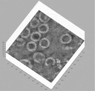
At this stage, looking at the deconvolved tomograms in any visualisation package (3dmod, dynamo_tomoslice, FIJI, napari) allows us to see that:
the VLPs are nearly spherical
proteins on the surface of the VLPs form a hexagonal lattice on the membrane
the lattice spacing is roughly 7.5 nm
We can use this information to help us in our efforts to reconstruct this lattice structure:
We can generate initial estimates for particle positions as points on a sphere centered on a VLP with the correct radius. These positions will be incorrect but particles extracted at these positions will contain our lattice structure.
The lattice is always parallel to the membrane, imparting an orientation normal to the surface of the sphere onto each particle will provide a consistent estimate for the initial orientation of the particles in the lattice.
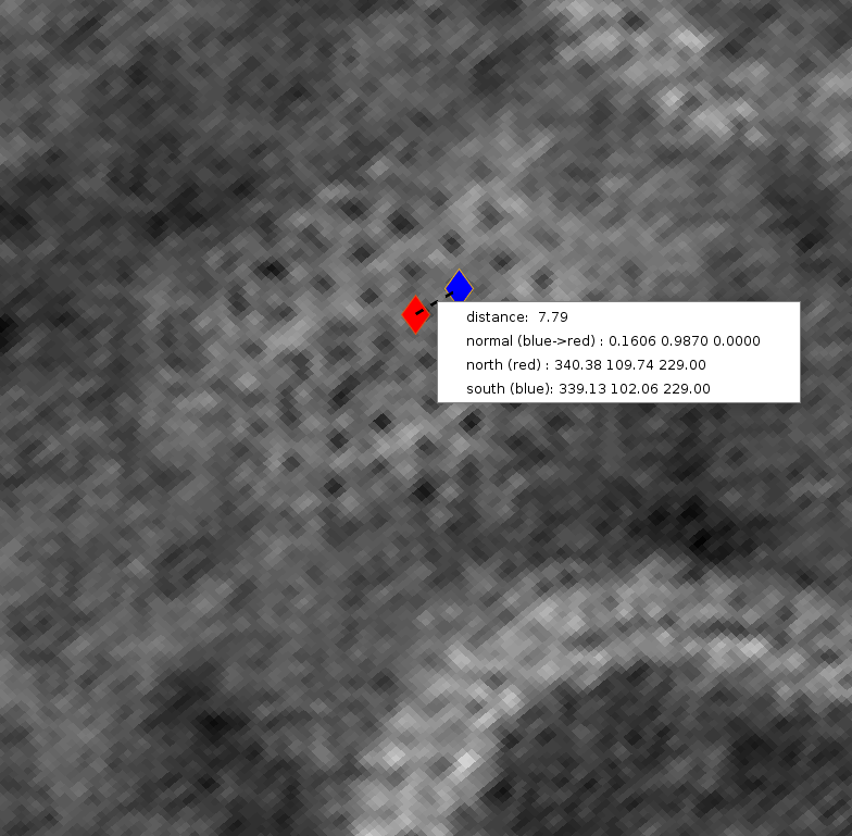
Dynamo contains many geometrical modelling tools which can help with these geometrical approaches to subtomogram averaging projects. We will make use of a limited subset of these tools in this tutorial, for an overview of the available geometrical models please see here. Becoming familiar with the available tools and thinking about how you can use the geometry of your system to your advantage will help with many subtomogram averaging projects. Below, we used dynamo_tomoslice to estimate the lattice spacing in our tomograms, 7.8 px at 10 Å/px this tool will be introduced shortly.
Generating a Dynamo catalogue for particle picking#
We now need a system for managing our reconstructed tomograms and annotations. A Dynamo catalogue is a database which facilitates the management of tomography data, including annotations and subsequent particle extraction.
We have provided a function warp2catalogue in the autoalign_dynamo package which will setup a catalogue from your Warp tomograms and their deconvolved counterparts. The catalogue is set up in such a way that any visualisation of the tomograms from the catalogue will display the deconvolved volumes but particles are extracted from the unfiltered volumes which are suitable for alignment and averaging experiments.
The function takes two arguments: the warp reconstruction directory and the pixel spacing of the reconstructed tomograms.
Let’s create a new dynamo folder in the project root directory, and navigate to it in Matlab. Then, we run:
warp2catalogue('../frames/reconstruction', 10)
This will generate the catalogue with the name warp_catalogue inside the dynamo directory. To open the catalogue manager in dynamo, run
dcm warp_catalogue
From the catalogue manager which opens up, tomograms can be opened in an interactive browser called dynamo_tomoslice by first selecting the tomogram of interest then using the View volume -> Open full volume with tomoslice menu options.
At this point we recommend getting comfortable with basic manipulation of the tomoslice viewer. As you can probably tell by the number of buttons and menus, this viewer contains many powerful tools. Don’t be scared! Read the wiki page describing how to use it. Once you feel comfortable, move onto the next section where we will annotate our VLPs to provide initial positions and orientations for subtomogram averaging.
VLP annotation#
Defining our approach#
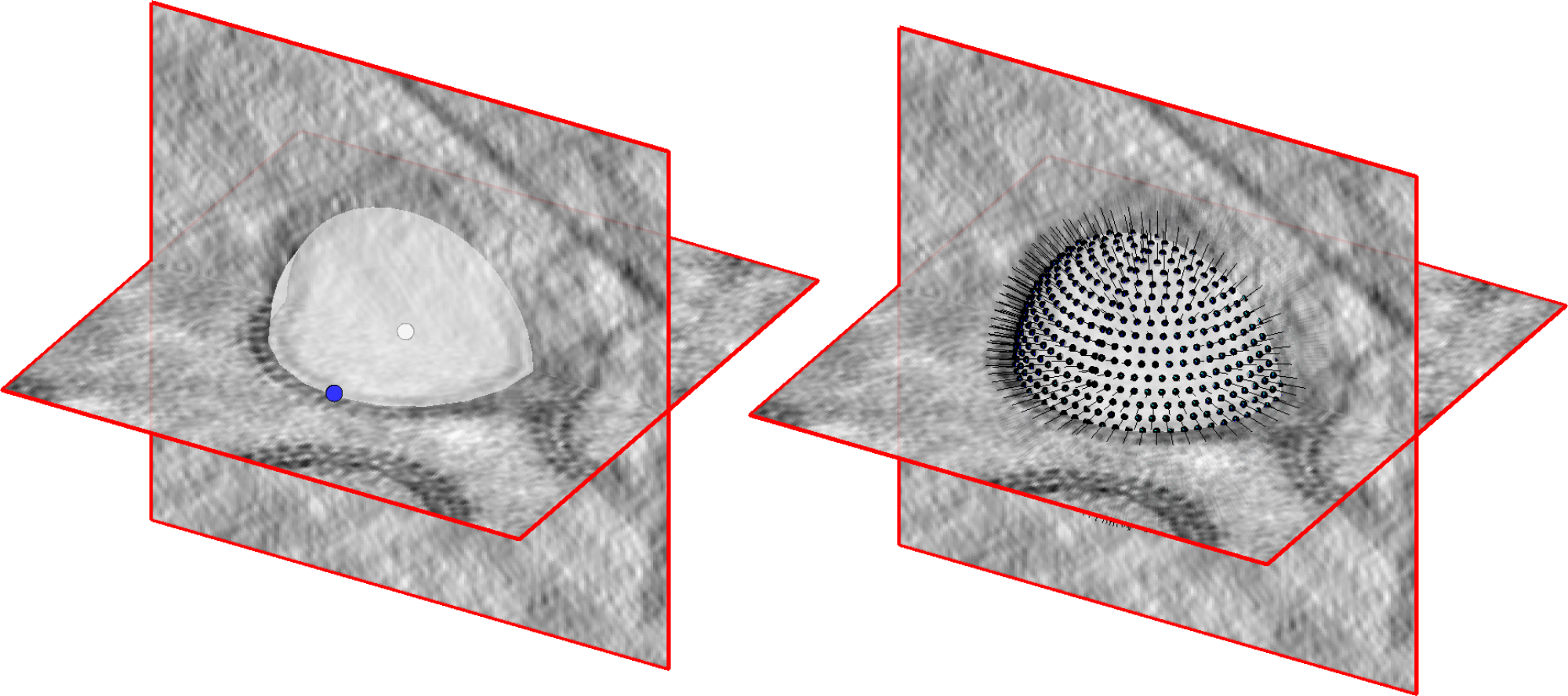
We need to annotate many spherical VLPs within each tomogram. Whilst we could achieve this by annotating each sphere as a vesicle model directly, the workflow for defining vesicle models from dynamo_tomoslice requires defining many points for each vesicle model. This approach is robust, but not especially quick if we have many annotations to make.
Instead, we will take a shortcut - spheres can be completely defined by only two values, their centre point and their radius. We will create a dipoleSet model in each tomogram to annotate the centres and edge points of many VLPs quickly in just one model, then convert these dipoleSet models into oversampled vesicles with a function which we provide.
Tomogram annotation#
Follow the guide for creating dipoleSet models and turning them into oversampled Vesicle models here.
Your expected inter-particle distance at this stage is ~7.5 nm, the lattice spacing we observed earlier.
Here’s a short video of us picking some vescicles on the TS_03 tomogram: